# Penser à installer les packages: pip install nom_package

import numpy  as np
import pandas as pd
import patsy  as pt
import lifelines as lf
import matplotlib.pyplot as plt
import statsmodels as sm18 Python
Le document qui suit n’est qu’un programme fait il y a 5 ans, et non repris depuis (mais ça marche. Utilisant très peu Python, je n’ai pas documenté les fonctions, qui ont été utilisées.
J’ai essayé de réglé tant bien que mal un bug d’affichage à partir de la proportionnalité des risques, qui conduisait à un affichage en pleine page. Cette section n’étant pas très développée, je n’ai pas trop insisté (l’accès à la table des matières n’est plus disponible sur la moitié du document).
Deux paquets d’analyse: principalement lifelines (km, cox, aft…) et `statsmodels``` (estimation logit en temps discret, kaplan-Meier, Cox).
Le package statsmodels est également en mesure d’estimer des courbes de séjour de type Kaplan-Meier et des modèles à risque proportionnel de Cox. Le package lifelines couvre la quasi totalité des méthodes standards, à l’exception des risques concurrents.
Le calcul des Rmst a été ajouté au package lifelines récemment. J’ai ajouté cette mise à jour.
Chargement de la base
trans = pd.read_csv("https://raw.githubusercontent.com/mthevenin/analyse_duree/master/bases/transplantation.csv")

trans.head(10)
trans.info()
<class 'pandas.core.frame.DataFrame'>
RangeIndex: 103 entries, 0 to 102
Data columns (total 10 columns):
# Column Non-Null Count Dtype
--- ------ -------------- -----
0 id 103 non-null int64
1 year 103 non-null int64
2 age 103 non-null int64
3 died 103 non-null int64
4 stime 103 non-null int64
5 surgery 103 non-null int64
6 transplant 103 non-null int64
7 wait 103 non-null int64
8 mois 103 non-null int64
9 compet 103 non-null int64
dtypes: int64(10)
memory usage: 8.2 KB18.1 Package lifelines
Documentation: https://lifelines.readthedocs.io/en/latest/
18.1.1 Non Paramétrique: Kaplan Meier
18.1.1.1 Calcul des estimateurs
Estimateur KM et durée médiane
T = trans['stime']
E = trans['died']


from lifelines import KaplanMeierFitter
kmf = KaplanMeierFitter()
kmf.fit(T,E)
print(kmf.survival_function_)
a = "DUREE MEDIANE:"
b = kmf.median_survival_time_
print(a,b)
KM_estimate
timeline
0.0 1.000000
1.0 0.990291
2.0 0.961165
3.0 0.932039
5.0 0.912621
... ...
1400.0 0.151912
1407.0 0.151912
1571.0 0.151912
1586.0 0.151912
1799.0 0.151912
[89 rows x 1 columns]
DUREE MEDIANE: 100.0kmf.plot()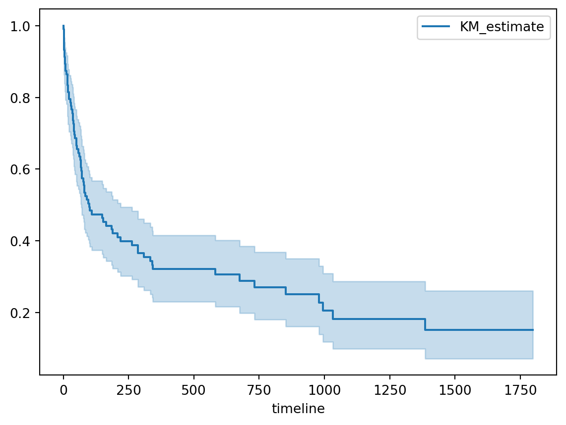
Comparaison des fonctions de survie
ax = plt.subplot(111)
kmf = KaplanMeierFitter()
for name, grouped_df in trans.groupby('surgery'):
    kmf.fit(grouped_df['stime'], grouped_df['died'], label=name)
    kmf.plot(ax=ax)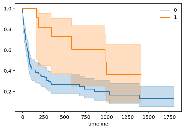
18.1.1.2 Tests du logrank
from lifelines.statistics import multivariate_logrank_test
results = multivariate_logrank_test(trans['stime'], trans['surgery'], trans['died'])
results.print_summary()| t_0 | -1 |
| null_distribution | chi squared |
| degrees_of_freedom | 1 |
| test_name | multivariate_logrank_test |
| test_statistic | p | -log2(p) | |
|---|---|---|---|
| 0 | 6.59 | 0.01 | 6.61 |
18.1.1.3 Calcul des Rmst
Note
- Update 2024.
- Programmation très lourde.
- Pas de test de comparaison des RMST (différence ou ratio).
- Chargement de la fonction
from lifelines.utils import restricted_mean_survival_time- Définition de la valeur du groupe exposé (ici surgery égal à 1)
ix = trans['surgery'] == 1- Définition de la durée maximale. Ici 1407 jours (idem R par défaut)
tmax = 1407- Calcul des Rmst
kmf_1 = KaplanMeierFitter().fit(T[ix], E[ix], label='Opérés')
rmst_1 = restricted_mean_survival_time(kmf_1, t=tmax)

kmf_0 = KaplanMeierFitter().fit(T[~ix], E[~ix], label='Non opérés')
rmst_0 = restricted_mean_survival_time(kmf_0, t=tmax)
Rmst pour surgery = 0
rmst_0379.14763007035475Rmst pour surgery = 1
rmst_1884.5757575757575- Courbes des Rmst pour tmax = 1407
from matplotlib import pyplot as plt
from lifelines.plotting import rmst_plot

ax = plt.subplot(311)
rmst_plot(kmf_1, t=tmax, ax=ax)

ax = plt.subplot(312)
rmst_plot(kmf_0, t=tmax, ax=ax)

ax = plt.subplot(313)
rmst_plot(kmf_1, model2=kmf_0, t=tmax, ax=ax)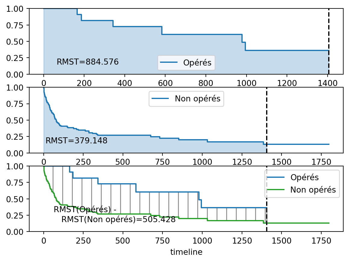
18.1.2 Semi paramétrique: Cox
18.1.2.1 Estimation
model = 'year + age + C(surgery) -1'
X = pt.dmatrix(model, trans, return_type='dataframe')
design_info = X.design_info
YX = X.join(trans[['stime','died']])
YX.drop(['C(surgery)[0]'], axis=1, inplace=True)
YX.head()
from lifelines import CoxPHFitter
cph = CoxPHFitter()
cph.fit(YX, duration_col='stime', event_col='died')
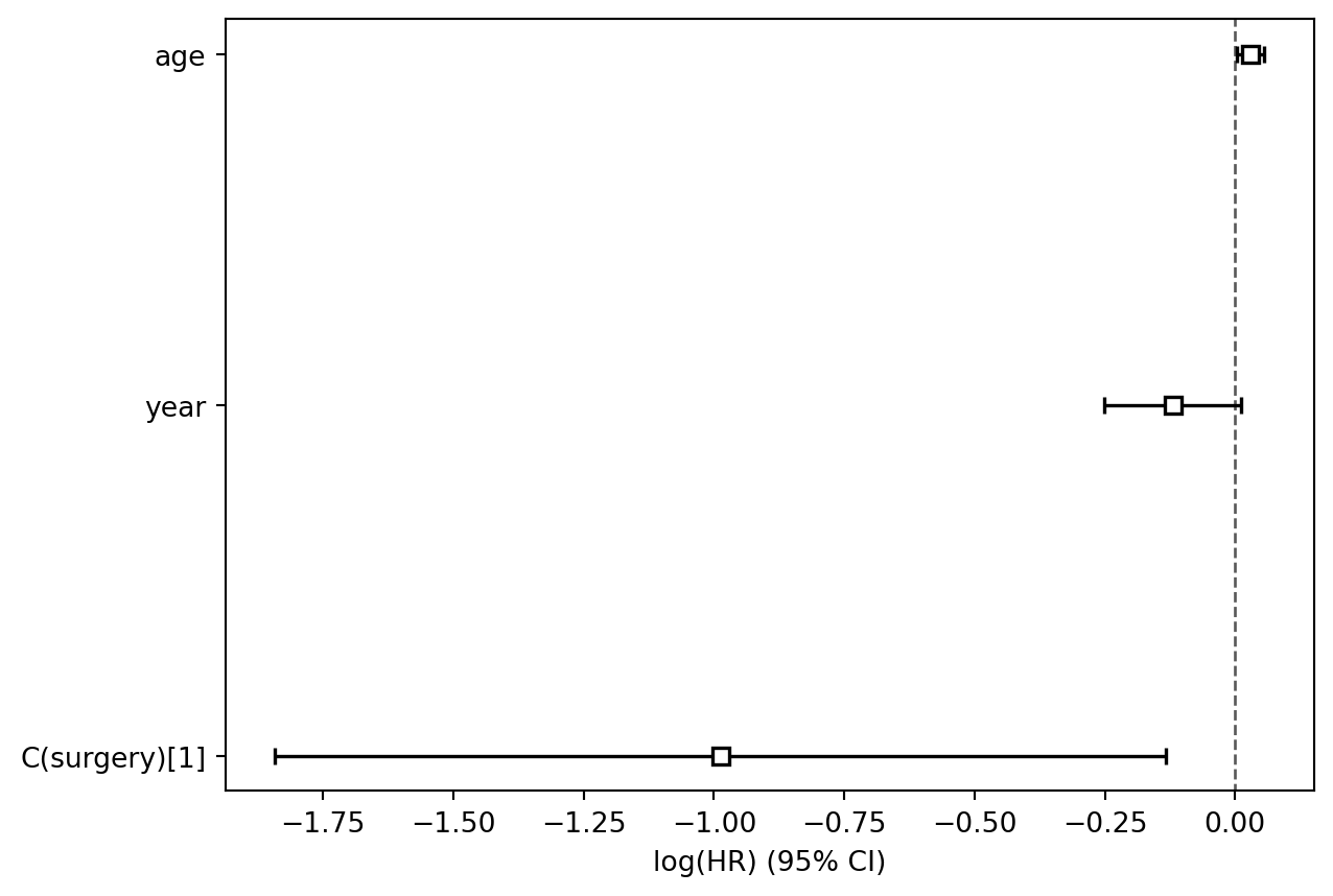
cph.print_summary()
cph.plot()| model | lifelines.CoxPHFitter |
| duration col | 'stime' |
| event col | 'died' |
| baseline estimation | breslow |
| number of observations | 103 |
| number of events observed | 75 |
| partial log-likelihood | -289.31 |
| time fit was run | 2024-09-24 06:52:44 UTC |
| coef | exp(coef) | se(coef) | coef lower 95% | coef upper 95% | exp(coef) lower 95% | exp(coef) upper 95% | cmp to | z | p | -log2(p) | |
|---|---|---|---|---|---|---|---|---|---|---|---|
| C(surgery)[1] | -0.99 | 0.37 | 0.44 | -1.84 | -0.13 | 0.16 | 0.88 | 0.00 | -2.26 | 0.02 | 5.40 |
| year | -0.12 | 0.89 | 0.07 | -0.25 | 0.01 | 0.78 | 1.01 | 0.00 | -1.78 | 0.08 | 3.72 |
| age | 0.03 | 1.03 | 0.01 | 0.00 | 0.06 | 1.00 | 1.06 | 0.00 | 2.19 | 0.03 | 5.12 |
| Concordance | 0.65 |
| Partial AIC | 584.61 |
| log-likelihood ratio test | 17.63 on 3 df |
| -log2(p) of ll-ratio test | 10.90 |